AlphaZero
A step-by-step look at Alpha Zero and Monte Carlo Tree Search
A simpler game
Go has ~2.08x10170 legal board positions. Chess has ~1050 legal board positions. Even Tic-Tac-Toe has 5,478 legal board positions. If we’re going to have any hope of understanding AlphaZero and MCTS for the first time, we’re going to need a simpler game. We need a super simple game that still allows for wins, losses and draws.
Ladies and gentlemen, for your consideration: Connect2!

In Connect2 players alternate between playing pieces on a tiny 1x4 board with the goal of placing two of their pieces side-by-side.
It’s comically easy to win as the first player, but Connect2 still has the interesting property that either player technically has the chance to win, lose or draw.
This means we can use it as a test bed to debug and visualize a super-basic implementation of AlphaZero and Monte Carlo Tree Search.
Below is the complete game tree of all 53 possible Connect2 states:
In total, there are 24 terminal states. From Player 1′s perspective there are:
- 12 terminal states where we WIN
- 8 terminal states where we LOSE
- 4 terminal states where we DRAW
Representing the Game
One drawback of AlphaZero is that we need to be able to perfectly simulate the game we want to play. This ends up being relatively straightforward for Connect2 but is much more difficult for games like chess that have more complex rules. The full code for Connect2 is available on GitHub. It contains logic that defines what moves are valid, how to transition between states and what reward a player should receive.
In our implementation we’re going to represent a player’s own pieces with 1, their opponent’s pieces with -1 and an empty space as 0. So the initial starting state looks like [0,0,0,0]. The player who wins the game will receive a reward of 1 and the player who loses will receive -1. Draws will receive a reward of 0.
Note: There is a very important detail here: The player who is playing always sees their own pieces as 1. In our implementation, we simply multiply the board by -1 every time we transition between players. Below, observe that state “toggles” as players take turns placing pieces:
AlphaZero
AlphaZero is built from three core pieces:
- Value Network
- Policy Network
- Monte Carlo Tree Search
Value Network
The value network accepts a board state as input and gives us a score as output. If we are going to win with absolute certainty, we want our value network to output 1. If we are going to lose, we want our value network to output -1. If we are going to draw, we want our value network to output 0.
For example, the game below is guaranteed to be a tie, so we’d like our network to produce 0 (or something close to it).
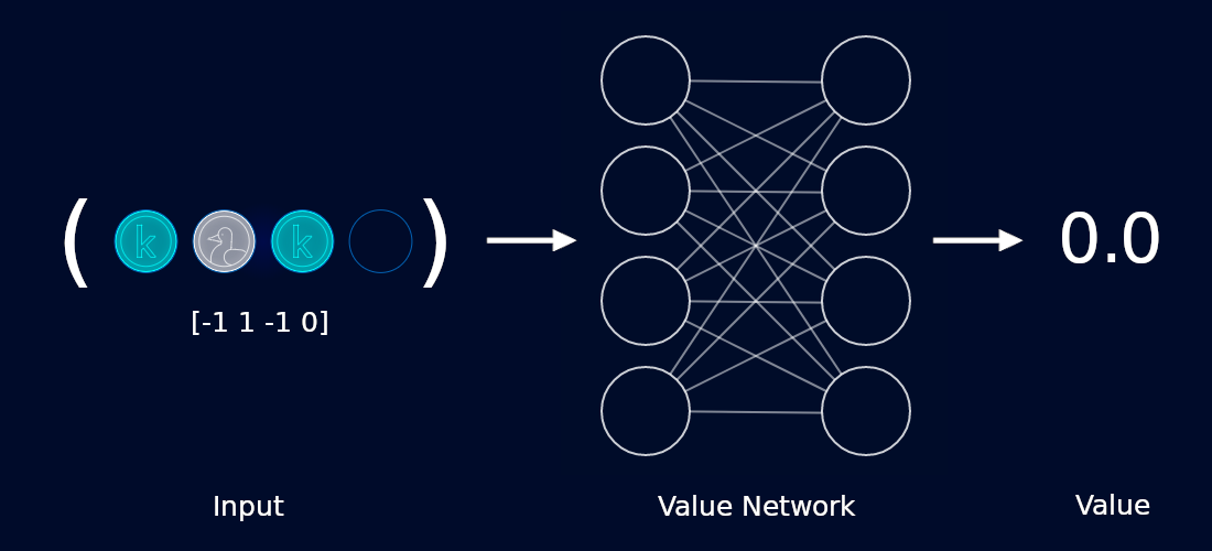
There are some subtleties here worth discussing. First off, our network isn’t doing any “thinking” to produce a value. That is, it’s not looking ahead, considering all possible moves or anything like that. It’s esssentially acting as an image classifier. In fact for 2D games like Go, we would borrow computer vision architectures like ResNet and use them as the backbone for our networks.
Training
In order to train this network, we need to record the moves taken by each player during a self-play game. For example, a sample game might look like:
[ 0  0  0  0]   # Player 1 plays in the first position
[-1  0  0  0]   # Player 2 plays in the third position
[ 1  0 -1  0]   # Player 1 plays in the second position
After the final move, Player 1 will be declared the winner. We go back through all the states held by Player 1 and mark them with a reward of
1. Similarily, we go through all the states held by Player 2 and mark them with a reward of -1.
Our recorded states would now look something like:
([ 0  0  0  0],  1)   # Player 1 plays in the first position
([-1  0  0  0], -1)   # Player 2 plays in the third position
([ 1  0 -1  0],  1)   # Player 1 plays in the second position
We collect this kind of state and reward information across a large number of games. We then use these recordings as a dataset to train our value network.
We ask our network how it would have “valued” a given state, and then train it to be closer to the actual value seen
(always 1,0 or -1,) when playing games. The hope is that with enough training, our value network will
start to value game states correctly.
It’s our hope that over a long enough time horizon, our value network will become increasingly good at identifying “good” states. This ends up being important as it will help guide our Monte Carlo Tree Search later.
Policy Network
The policy network accepts a board state as input and gives us a set of probabilities for each move as output. The “better” the move, the higher we would like the probability for the corresponding position. The role of the policy network is to “guide” our Monte Carlo Tree search by suggesting promising moves. The Monte Carlo Tree Search takes these suggestions and digs deeper into the games that they would create (more on that later).
We call the suggestions produced by the policy network “priors”.
For example, the game below can be won in a single move, so we’d like our network to confidently suggest that we play in the first position:
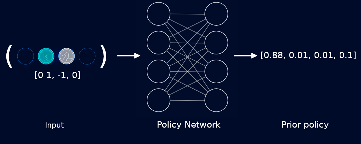
Note that our network often gives non-zero probabilities to illegal moves. Above, our network gives 0.01 to the second and third slots. We actually have to correct for this manually by masking out illegal moves, and then re-normalizing the remaining scores so they still sum to a probability of 1.00.
Like the value network, our policy network is not doing any kind of “deep thinking” or lookahead. In fact it’s more comparable to something like a human playing bullet chess. It’s simply making a snap decision based on the current state of the board.
Training
One thing I found counter-intuitive about AlphaZero is that we don’t directly train our policy network to make “good” moves. Instead we train it to mimic the output of the Monte Carlo Tree Search. As we play games, the policy network suggests moves to Monte Carlo Tree Search. MCTS uses these suggestions (or priors) to explore the game tree and returns a better set of probabilities for a given state. We record the state and the probabilities produced by the MCTS. For example, a sample game might look like:
([ 0  0  0  0], [0.1, 0.4, 0.4, 0.1])
([-1  0  0  0], [0.0, 0.3, 0.3, 0.3])
([ 1  0 -1  0], [0.0, 0.8, 0.0, 0.2])
Once again, we collect this information over a large number of games. We use these recordings as a dataset to train our policy network. We ask our policy network what prior probabilities it would recommend for a given state. We then use Cross Entropy Loss to try and match the policy network’s priors to the probabilities recommended by the MCTS.
Monte Carlo Tree Search
Despite the world’s focus on the neural networks involved in AlphaZero, the true magic of AlphaZero actually comes from Monte Carlo Tree Search. It’s here that AlphaZero simulates moves and looks ahead to explore a range of promising moves.
The search tree we’re using is the same as the ones shown above. Each node represents a reachable board state and the edges represent actions that a player can take in that state. Each node stores a few pieces of information on it:
class Node:
  def __init__(self, prior, to_play):
      self.prior = prior      # The prior probability of selecting this state from its parent
      self.to_play = to_play  # The player whose turn it is. (1 or -1)

      self.children = {}      # A lookup of legal child positions
      self.visit_count = 0    # Number of times this state was visited during MCTS. "Good" are visited more then "bad" states.
      self.value_sum = 0      # The total value of this state from all visits
      self.state = None       # The board state as this node

  def value(self):
       # Average value for a node
      return self.value_sum / self.visit_count
Starting with an empty tree, Monte Carlo Tree Search iteratively builds up a portion of the game tree by running a number of “simulations”. Each simulation adds a single node to the game tree and consists of three stages:
- Select
- Expand
- Backup
Generally, the more simulations we run, the better we can expect our model to play. When playing Go, AlphaZero was configured to run 1,600 simulations per move.
Before we try to understand each stage, let’s watch Monte Carlo Tree Search in action to try to get a feel for how it all works. Below we run only five simulations to build up a small portion of the overall game tree.
Note: In the below simluation we have hard-coded our policy network to output equal priors for every move (that is, it says every move looks equally promising) and an arbitrary value of 0.5 for every position.
def run(self, state, to_play, num_simulations=5):
    root = Node(0, to_play)
    # EXPAND root
    root.expand(self.model, self.game, state, to_play)

    for _ in range(num_simulations):
        node = root
        search_path = [node]
        # SELECT
        while node.expanded():
            action, node = node.select_child()
            search_path.append(node)

        parent = search_path[-2]
        state = parent.state
        next_state, _ = self.game.get_next_state(state, to_play=1, action=action)
        next_state = self.game.get_canonical_board(next_state, player=-1)
        value = self.game.get_reward_for_player(next_state, player=1)
        if value is None:
            # EXPAND
            value = node.expand(self.model, self.game, next_state, parent.to_play * -1)

        self.backup(search_path, value, parent.to_play * -1)

    return root
Now that we’ve watched Monte Carlo Tree Search, let’s break down what’s actually going on here. We start by creating a root node for the current state of the board and “Expanding” it. When we expand a node, we ask our policy network to give us a list of prior probabilities for every possible move we could make. We then add these possible moves as child nodes to the current node. We haven’t actually explored these child nodes, we just know that we are legally allowed make these moves and they will bring us to some unknown state.
After expanding the root node, we begin our very first MCTS simulation. Our goal here is to find an unvisited leaf node and EXPAND it. But how do we choose which nodes to visit? We greedily select the child node with the highest “Upper Confidence Bound (UCB) Score”.
UCB Score attempts to take three things into account when producing a score:
- The prior probability for the child action
- The value for the state the child action leads to
- The number of times we’ve taken this action in past simulations
def ucb_score(parent, child):
    prior_score = child.prior * math.sqrt(parent.visit_count) / (child.visit_count + 1)
    if child.visit_count > 0:
        # The value of the child is from the perspective of the opposing player
        value_score = -child.value()
    else:
        value_score = 0

    return value_score + prior_score
We repeatedly select child nodes using UCB Score to guide our search and use search_path to keep track of the nodes we’ve visited.
Once we reach a leaf node, we check whether or not the game has ended. If the game is complete we don’t need to expand this leaf node.
If the game is not complete, we expand the leaf node the same way as before: We ask the policy network for a set of priors and assign those to the newly created nodes.
After expanding the node, we enter the last stage of our MCTS simluation: Backup. In this stage, we update the statistics (visit_count and value_sum) for
every node in the search_path. Updating these statistics will change their UCB score, and guide our next MCTS simulation.
After we’ve run the maximum number of simulations, we return the root of the game tree. The child of this root with the highest visit count is the “best” action. If we’re playing competitively this is probably the action we want to take. If we’re training, we usually want to encourage more exploration and instead use the visit counts to create a probability distribution that we can sample from. The best moves is still likely to be selected, but it gives our model the opportunity to explore other moves.
More resources
AlphaZero Simple - Code on GitHub
Mastering the game of Go without human knowledge
Mastering Chess and Shogi by Self-Play with a General Reinforcement Learning Algorithm